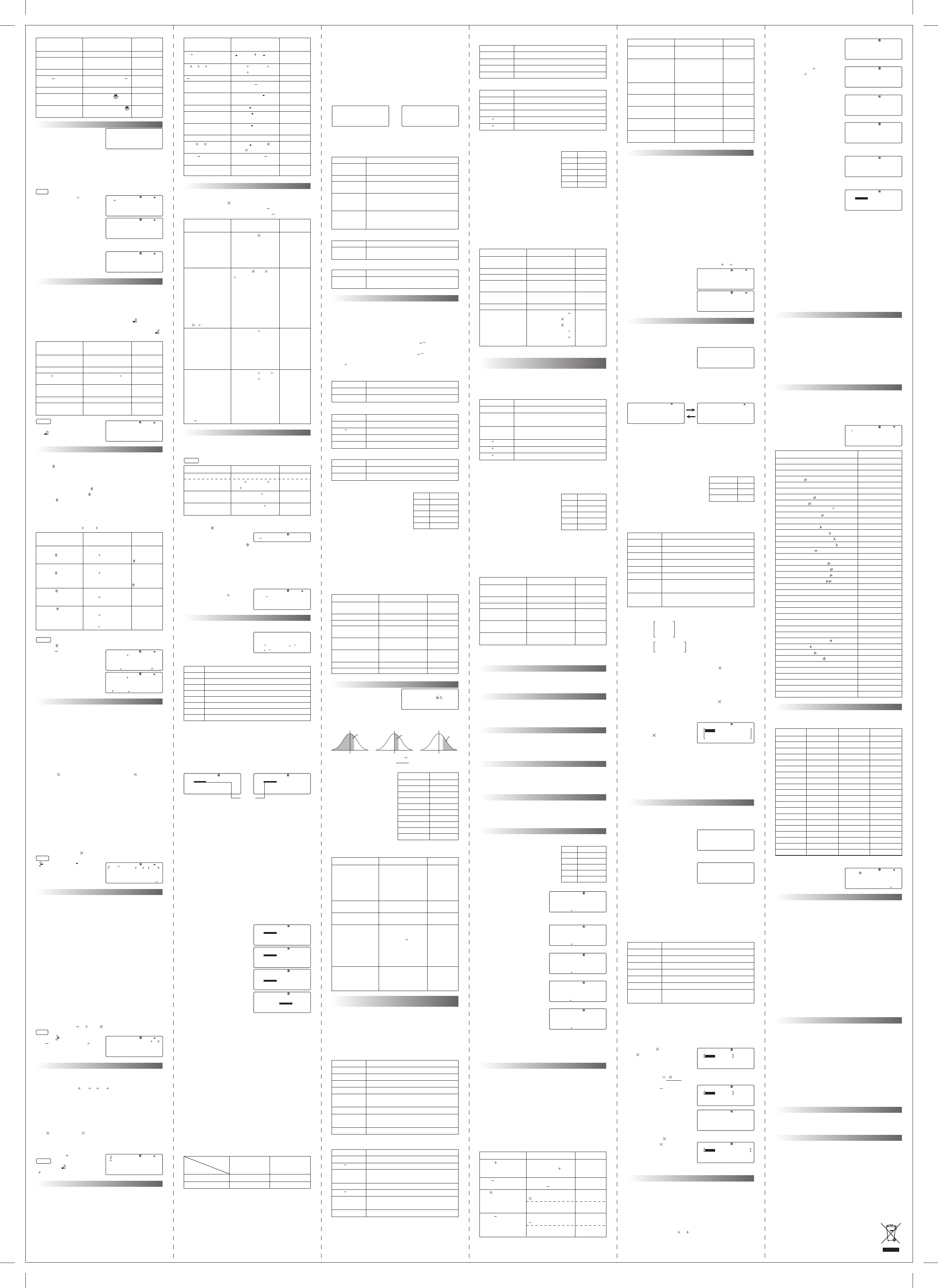
STAT Calculation Screen
Pressing the [AC] key while the STAT editor screen is displayed
switches to the STAT calculation screen to perform statistical
calculations. This screen uses linear format regardless of the
current input/output format setting on the calculator’s setup
screen.
STAT Menu
While the STAT editor screen or STAT calculation screen is on
the display, press [SHIFT] [1] to display the STAT menu. The
contents of the STAT menu for a single or paired variables are
different and are shown below:
The following tables explain the key function of the STAT
menu
Common items:
The following is only available in the single-variable statistics
The following is only available in the paired-variable statistics
Single-variable Statistical Calculation
The following are th
e commands that appear on the
sub-menus that appear when you select [3] (Sum), [4] (Var), or
[6] (MinMax) on the STAT menu while a single-variable
statistical calculation type is selected.
Standard deviation and mean calculations are performed as
shown below:
Population standard deviation xσn = √(∑(x
i
x)
2
/n)
where i = 1 to n
Sample standard deviation xσn–1 = √(∑(x
i
x)
2
/(n-1))
where i = 1 to n
Mean x = (∑x)/n
Sum Sub-menu ( [SHIFT] [1] [3] )
Var Sub-menu ( [SHIFT] [1] [4] )
MinMax Sub-menu ( [SHIFT] [1] [6] )
Example
Use these data to calculate:
Sum of squares of the sample data
Sum of the sample data
Number of samples
Mean of the sample data
Population standard deviation
Sample standard deviation
Minimum value
Maximum value
Press [SHIFT] [MODE] [] [4] [1] to turn on the “Frequency
Column”.
Press [MODE] [3] [1] to select single-variable (1-VAR)
Input the data:
[5] [5] [=] [5] [4] [=] [5] [2] [=] [5] [1] [=] [5] [3] [=]
[] [] [2] [=] [2] [=] [] [] [2] [=]
Press [AC]
Probability Distribution Calculation (Distr sub-menu)
You can calculate probabiltiy
distributions for single-variable
statistics by pressing [SHIFT]
[1] [5] in the STAT mode.
Input a value from 1 to 4 to select the probabilty distribution
calculation you want to perform.
Example: This table shows
the results of measurements
of the height of 20 college
students. Determine what
percentage of the students
fall in the range of 160.5cm
to175.5cm. Also, in what
percentile does the 175.5cm
tall student fall?
Input the data using the
STAT Editor Screen with
the Frequency Column “ON”
Then you can perform the calculations.
Commands when Linear Reg
ression Calculation (A+BX) is
Selected
Linear regression calculations are carried out using the
following formula:
y = A + Bx.
The following are the commands that appear on the
sub-menus that appear when you select [3] (Sum), [4] (Var), [6]
(MinMax), or [5] (Reg) on the STAT menu while linear
regression is selected as the statistical calculation type.
Sum Sub-menu ( [SHIFT] [1] [3] )
Var Sub-menu ( [SHIFT] [1] [4] )
Degree, Radian, Gradient Interconversion
Degree, radian and gradient
can be converted to each other
with the use of [SHIFT] [Ans]
( i.e. DRG). After inputting
a value, press [SHIFT] [Ans] to display the angle unit
specification menu. Press the number key that corresponds to
the angle unit of the input value.
The calculator will
automatically convert it to the calculator’s default angle unit.
Example 1: To convert the following value to degrees:
π/4 = 45
º
, 60 grads = 54
º
, angle unit: Deg
LINE
[ ( ] [SHIFT] [x10
x
] [ ] [4] [ ) ]
[SHIFT] [Ans] [2] [=]
[6] [0] [SHIFT] [Ans] [3] [=]
Example 2: cos(π radians) = –1
[cos] [SHIFT] [x10
x
]
[SHIFT] [Ans] [2] [ ) ] [=]
Logarithmic and Exponential Functions
• For the logarithmic function ( [log] ), you can specify base m
using the format “log (m, n)”. Example: log
2
30 Press [log] [2]
[SHIFT] [ ) ] [3] [0] [ ) ] [=]
If you input only a single value, base 10 is the default.
Example: log
10
16 Press [log] [1] [6] [ ) ] [=]
• [In] is a natural logarithm function with base e.
• In Math format you can also use the [log ] key when
inputting an expression with the form of “logmn”. However,
you must input the base (base m) when using the [log ]
function key.
MATH
log
2
16 = 4
[log ] [2] [] [1] [6] [=]
Coordinate Transformation
• This scientific calculator lets you convert between
rectangular coordinates and polar c
oordinates, i.e., P(x, y) ↔
Rec(r, )
• Coordinate transformation can be performed in the COMP
and STAT calculation modes.
• Calculation results x and r are stored in variable memory X.
Calculation results y and
are stored in variable memory Y.
• With polar coordinates, can be calculated within a range of
–180
º
<
≤
180
º
.
• If you perform coordinate transformation inside of an
expression instead of a stand alone operation, the
calculation is performed using only the first value (either the
r-value or the x-value) produced by the transformation.
Example: Pol( 2, 2)
5 = 2 5 = 7
MATH
r=25 and
= 56
º
, what are x and y? (Angle unit : Deg)
[SHIFT] [ ] [2] [5] [SHIFT]
[ ) ] [5] [6] [ ) ] [=]
Press [] repeatedly until the
right arrow disappears to show
the full value of Y.
Integration Calculation
Integration calculation is performed using Gauss-Kronrod
method of numerical integration.
∫ ( f (x), a, b, tol )
f (x): Function of X (all non-X variables are treated as
constants)
a: Integration interval lower limit
b: Integration interval upper limit
tol: Tolerance range (input / output format: Linear)
• Although a smaller tol value provides better precision, it
causes the calculation to take more time. Specify a tol value
that is 1
10
–14
or greater. A default value of 1
10
–5
is used
when you omit specification of the tolerance range.
• Integration calculations can be performed in the COMP
Mode only.
• Specify Rad as the calculator’s default angle unit, when
performing an integration calculation involving
trigonometric functions.
• Integration calculations can take considerable time to
complete.
• You cannot input a tol value when using Math format.
• Errors may occur due to the type of function being
integrated, the presence of positive and negative values in
the integration interval, or the interval.
Example: ∫ ( x
–2
, 5, 1, 1 10
–7
) = –0.8
LINE
[∫ ] [ALPHA] [ ) ] [x ] [ (–) ] [2]
[ ) ] [SHIFT] [ ) ] [5] [SHIFT] [ ) ]
[1] [SHIFT] [ ) ] [1] [x10
x
]
[ (–) ] [7] [ ) ] [=]
Differential Calculation
Your calculator performs differential calculations by
approximating the derivative based on centered difference
approximation.
d/dx ( f (x), a, tol )
f (x): Function of X (all non-X variables are treated as
constants)
a: Input a value to specify the point for which the
derivative should be obtained (differential point)
tol: Tolerance range (input / output format: Linear)
• Inaccurate results and errors can be caused by the
following:-
- discontinuous points in x values
- extreme changes in x values
- inclusion of the total maximum point and local minimum
point in x values
- inclusion of the inflection point in x values
- inclusion of undifferentiable points in x
values
- differential calculation results approaching zero
• Other limitations as stated for Integration Calculations also
applied in Differential Calculations.
Example: d/dx ( 3x
2
5x 2, 2, 1 10
–12
) = 7
LINE
[SHIFT] [∫ ] [3] [ALPHA] [ ) ]
[x
2
][ ] [5] [ALPHA] [ ) ] [ ] [2]
[SHIFT] [ ) ] [2] [SHIFT] [ ) ]
[1] [x10
x
] [ (–) ] [1] [2] [ ) ] [=]
∑ Calculations
With ∑(, you can obtain the sum of an input f(x) expression for
a specific range. ∑ calculaions are performed using the
following
∑ ( f (x), a, b ) = f (a)
f (a 1) ...... f (b)
f (x): Function of X (all non-X variables are treated as
constants)
a: Calculation range start point
b: Calculation range end point
• a and b are integers in the range of
–1
10
10
< a ≤ b < 1
10
10
• The calculation step is fixed at 1
•
∫(, d/dx(, Pol(, Rec(, and ∑( cannot be used within f (x), a or b
Example: ∑ ( X 2, 1, 5 ) = 25
MATH
[SHIFT] [log ] [ALPHA] [ ) ]
[
] [2] [] [1] [] [5] [=]
Other Functions
Factorial (!) function obtains the factorial of a value that is
zero or a positive integer.
Absolute Value Calculation (Abs) obtains the absolute value
when you are performing a real number calculation.
Random Number (Ran#) generates a 3-digit pseudo random
number that is less than 1 (number is in the range of 0.000 to
0.999). Note that the values shown below are example only.
Values actually generated by your calculator will be different.
Permutation and Combination
These functions make it possible to perform permutation and
combination calculations. n and r must be integers in the
range of 0 ≤ r ≤ n ≤ 1
10
10
.
Total number of permutations nPr = n!/(n r)!
Total number of combinations nCr = n!/(r!(n
r)!)
Complex Number Calculation
• Press [MODE] [2] to enter the "CMPLX" mode for
calculations that include complex numbers.
• In the CMPLX Mode, the [ENG] key changes function to
become an imaginary number i input key.
MATH
• You can also input complex numbers using polar coordinate
format (r ∠
).
Example: To input 5∠30
[5] [SHIFT] [ (–) ] [3] [0]
• The angle unit for argument
input and result display is the
calculator’s default angle unit.
• At the end of the calculation, press [SHIFT] [2] [4] to specify
rectangular coordinate format for the calculation result.
• At the end of the calculation, press [SHIFT] [2] [3] to specify
polar coordinate format for the calculation result.
• To obtain a conjugate complex number press [SHIFT] [2] [2].
Example: To determine the conjugate of the complex
number 2+3i.
[SHIFT] [2] [2] [2] [
] [3] [i]
[ ) ] [=]
Statistical Calculations
All calculations in this section are performed in the STAT
Mode ( [MODE] [3] ).
Press [MODE] [3] to display
the STAT menu for statistical
calculation type selection.
There are eight types of statistical calculations.
Inputting Sample Data
Once you enter the STAT mode the STAT editor screen appears.
Select a statistical calculation type by pressing the
corresponding number. To display the STAT editor screen from
another STAT mode screen, press [SHIFT] [1] [2].
STAT Editor Screen
There are two STAT editor screen formats, depending on the
type of statistical calculation you selected.
• The first line of the STAT editor screen shows the value for the
first sample or the values for their first pair samples and the
second line shows the value of second sample and so on.
Frequency Column
A column
labeled “FREQ” will also be included on the STAT
editor screen if you turn on the Statistical Display item on the
calculator’s setup screen. You can use the FREQ column to
specify the frequency of each sample value.
Inputting Sample Data
• Data is inserted into the cell where the cursor is located. Use
the cursor keys to move the cursor between cells.
• The values and expressions you can input on the STAT editor
screen are the same as those you can input in the COMP
mode with Linear format.
• Pressing [AC] while inputting data clears your current input.
• After inputting a value, press [=] to confirm. This registers the
value but the cell can only display a maximum of 6 digits.
Example: To input the value 357 in cell X1, 8 in cell Y1.
[SHIFT] [1] [2]
(to display the STAT
editor screen)
[3] [5] [7]
(the value you input appears
in the formula area)
[=]
(registering a v
alue causes the
cursor to move down one cell)
[] [] [8] [=]
Editing Sample Data in the STAT Editor Screen
• Move the cursor to the cell you want to edit, input the new
data or expression then press [=]. Note that you must totally
replace the existing data of the cell with new input. You
cannot edit part of the existing data.
• To delete a line, move the cursor to the line you want to
delete, press [DEL].
• To insert a line, move the cursor to the line that will be under
the line you will insert, press [SHIFT] [1] [3] [1]. The insert
operation will not work if the maximum number of lines
allowed for the STAT editor screen are already used.
Deleting All Stat Editor Contents
Press [SHIFT] [1] [3] [2]
• You can only “insert a line” and “delet
e all stat editor contents”
when the STAT editor screen is on the display.
Notes
• The number of lines in STAT editor screen (the number of
sample data values you can input) depends on the type of
statistical data you selected, and on the “STAT” setting of the
calculator’s setup screen.
• To display the “STAT” setting screen press [SHIFT] [MODE]
[] [4].
• The following types of input are not allowed on the STAT
editor screen: [M+] , [SHIFT] [M+] , [SHIFT] [RCL] (i.e. “STO”).
• When you change to another mode from the STAT mode or
change the Statistical Display Setting (which enable or
disable the FREQ column) on the calculator’s setup screen, all
the sample data you input is deleted automatically.
Press [MODE] [7]
(select “TABLE”)
Input the function
[ALPHA] [ ) ] [
x
2
] [ ] [3]
[ALPHA] [ ) ] [ ] [3]
After making sure the function is correct, press
[=]
This displays the start value
input screen. (Initial default
start value is 1)
Press [3] [=] to specify the
initial start value for this
example. This displays the
end value input screen. (Initial
default end value is 5)
Press [7] [=] to specify the
end value for this example.
This displays the step value
input screen. (Initial
default step value is 1)
Press [2] [=] to specify the
step value for this example.
A number table is generated.
Pressing the [AC] key returns to the function editor screen.
Function Types that are supported
• Except for the X variable, other variables (A, B, C, D, Y) and
independent memory (M) are all treated as values (the
current variable assigned to the variable or stored in
independent memory).
• Only variable X can be used as the variable of a function.
• An error occur when an End value is less than Start value and
therefore the number table is not generated.
• Executing
a number generation table using a Start, End and
Step value combination that produces more than 30 x-values
causes an error. To avoid this, the specified Start, End, and
Step values should onlyproduce a maximum of 30 x-values.
• Certain functions and Start, End, Step value combinations can
cause number table generation to take a long time.
Number Table Screen
The number table screen shows x-values calculated using the
specified Start, End, and Step values, as well as the values
obtained when each x-value is substituted in the function f(x).
• Table contents cannot be edited. You can use the number
table screen for viewing values only.
• To returns to the function editor screen, press the [AC] key.
Note that in the Table Mode you should not change the
input/ouput format settings (Math format or
Linear
format) otherwise the number table generation function is
cleared.
Scientific Constants
A total of 40 commonly used scientific constants, such as the
speed of light in a vaccum and Planck's constant are built-in for
quick and easy look-up. Simply press [SHIFT] [7] and the
number that corresponds to the scientific constant (see the
table below for a complete list of available constants) you want
to look-up and press [=], it appears instantly on the display.
Example:
Press [SHIFT] [7] [2] [8] [=]
Metric Conversion
A total of 20 different conversion pairs a
re bulit-in to provide
quick and easy conversion to and from metric units. For details,
please refer to the following table.
Example: To convert 31 inches to centimeters
[3] [1] [SHIFT] [8] [0] [1] [=]
Trouble Shooting
Perform the following steps whenever an error occurs during a
calculation or when calculation results are not what you
expected. If one step does not correct the problem, move on to
the next step.
Note that you should make separate copies of important data
before performing these steps.
• Check the calculation expression to make sure that it does
not contain any errors.
• Make sure that you are using the correct mode for the type of
calculation you are trying to perform.
• If the above steps do not c
orrect your problem, press the
[ON] key. This will cause the calculator to perform a routine
that checks whether calculation functions are operating
correctly. If the calculator discovers any abnormality, it
automatically initializes the calculation mode and clears
memory contents.
• Initialize all modes and settings by performing the following
operation:
[SHIFT] [9] [1] [=]
Replacing the Battery
Dim figures on the display of the calculator indicate that
battery power is low. Continued use of the calculator when the
battery is low can result in improper operation. Replace the
battery as soon as possible when displ
ay figures become dim.
To replace the battery:-
• Remove the two screws that hold the back cover in place and
then remove the back cover,
• Remove the old battery,
• Wipe off the side of the new battery with a dry, soft cloth.
Load it into the unit with the positive(+) side facing up.
• Replace the battery cover and secure it in place with the two
screws.
• Press [ON] to turn power on.
Auto Power Off
Calculator power automatically turns off if you do not perform
any operation for about six minutes. When this happens, press
[ON] to turn power back on.
Specifications
Power supply: single LR44 battery
Operating temperature: 0
º
~ 40
º
C (32
º
F ~ 104
º
F)
MinMax Sub-menu ( [SHIFT] [1] [6] )
Reg Sub-menu ( [SHIFT] [1] [5] )
Example
Using this table, the regression
formula and correlation coefficient
can be obtained. Based on the
coefficient formula, the length of
the steel bar at 18ºC and the
temperature at 1000mm can be
estimated. Furthermore the critical
coefficient (r
2
) and covariance can
also be calculated.
Press [SHIFT] [MODE] [] [4] [2] to turn off the “Frequency
Column”.
Press [MODE] [3] [2] to select Linear regression (A+BX)
Input the data:
[1] [0] [=] [1] [5] [=] [2] [0] [=] [2] [5] [=] [3] [0] [=]
[] [] [1] [0] [0] [3] [=] [1] [0] [0] [5] [=]
[1] [0] [1] [0] [=] [1] [0] [1] [1] [=] [1] [0] [1] [4] [=]
Press [AC]
Commands when Quadratic Regression Calculation
(_+CX
2
) is Selected
Quadratic regression calculations are carried out using the
following formula:
y = A + Bx + Cx
2
Reg Sub-menu ( [SHIFT] [1] [5] )
• Sum sub-menu, Var sub-menu, and MinMax sub-menu
operations are the same as those for linear regression
calculations.
Example
Through quadratic regression of the
these data, the regression formula
and
correlation coefficient are
obtained. Furthermore, the
regression formula is used to
obtain the respective estimated
values of y and x, when
xi = 16 and yi = 20.
Press [SHIFT] [MODE] [] [4] [2] to turn off the “Frequency
Column”.
Press [MODE] [3] [3] to select Quadratic regression (_+CX
2
)
After using the method in the previous section to input the
data and now you can start the calculation.
You can use the above operating procedure for other types of
regression.
Logarithmic Regression
Logarithmic regression calculations are carried out using the
following formula:
y = A + Blnx
e Exponential Regression
e exponential regression calculations are carried out using the
following formula:
y = A
e
Bx
ab Exponential Regression
ab exponential regression calculations are carried out using
the following formula:
y = AB
x
Power Regression
Power regression calculations are carried out using the
following formula:
y = A
x
B
Inverse Regression
Power regression calculations are ca
rried out using the
following formula:
y = A + ( B/x )
Comparison of Regression Curves
Using the data input in the
example under “Linear
Regression Calculation” to
compare the correlation coefficient
for logarithmic, e exponential,
ab exponential, power and
inverse regression.
Correlation coefficient for logarithmic regression
Press [SHIFT] [1] [1]
(to select “Type”)
Press [4] [AC]
[SHIFT] [1] [5] [3] [=]
Correlation coefficient for e exponential regression
Press [SHIFT] [1] [1] [5] [AC]
[SHIFT] [1] [5] [3] [=]
Correlation coefficient for ab exponential regression
Press [SHIFT] [1] [1] [6] [AC]
[SHIFT] [1] [5] [3] [=]
Correlation coefficient for power regression
Press [SHIFT] [1] [1] [7] [AC]
[SHIFT] [1] [5] [3] [=]
Correlation coefficient for inverse regression
Press [SHIFT] [1] [1] [8] [AC]
[SHIFT] [1] [5] [3] [=]
Note: The commands included in the Reg sub-menu can take a
long time to execute in logarithmic, e exponential, ab
exponential, or power regression calcula
tion when there are a
large number of data samples.
BASE-N Calculations
The BASE-N Mode lets you perform arithmetic calculations,
negative value calculations, and logical operations with binary,
octal, decimal, and hexadecimal values.
• Press [SHIFT] [3] to display page one of the BASE menu
which lets you to input a negative number or logical
operation command. Logical operations are performed
through logical products (and), logical sums (or), negative
(Not), exclusive logic sums (xor), and negation of exclusive
logical sums (xnor).
• Press [SHIFT] [3] [] to display page two of the BASE menu
which lets you specify the number base. The number system
(10 [DEC], 16 [HEX], 2
[BIN], 8 [OCT]) is set by pressing [1], [2],
[3], [4] respectively. A corresponding symbol "d", "h", "b" or
"o" appears on the display.
Key Description
[1] (n) Number of samples
[2] (x) Mean of the X-data
[3] (x
σn) Population standard deviation of the
X-data
[4] (x
σn–1) Sample standard deviation of the X-data
[5] (y) Mean of the Y-data
[6] (y
σn) Population standard deviation of the
Y-data
[7] (y
σn–1) Sample standard deviation of the Y-data
Equation Solving Function
All calculations in this section are performed in the “EQN
Mode” ( [MODE] [5] ).
Four choices are provided for users to select. Press the
corresponding number to select the type of equation.
[1] 2-unknown simultaneous linear equations
[2] 3-unknown simultaneous linear equations
[3] Quadratic equation
[4] Cubic equation
• After selecting the type of equation, a coefficient editor
screen appears. Input all the coefficient respectively to solve
the equation.
• You can use [] and [] to switch the display between the
solutions for X and Y (and Z) in simultaneous linear
equations. Likewise, you can use [] and [] to scroll the
display between X
1, X2 and X3 in quadratic or cubic equation.
The actual number of solutions depends on the equation.
Example :- To solve the quadratic equation
x
2
2x 3=0
[MODE] [5] [3]
[1] [=] [2] [=] [3] [=]
[=]
[]
Matrix Calculations
Press [MODE] [6] to select the MATRIX MODE. You can save
matrices under the names “MatA”, “MatB”, “MatC” in matrix
memory. Matrix calculation results are stored in a special
Matrix Answer Memory named “MatAns”.
• In the MATRIX mode,
press [SHIFT] [4] [1] to
display the matrix selection
screen.
Note that the matrix selection screen also appears whenever
you enter the MATRIX mode.
• Press [1], [2] or [3] to specify the name of the matrix you
want to select. This display a screen for configuring
dimension settings. Press [] to display the second page of
dimension settings.
Press the corresponding number to spec
ify the matrix
dimension you want to use and the matrix editor screen
appears.
• Use the matrix editor screen to input each of the elements
into the matrix.
• If you want to create another matrix, repeat the above
procedure.
To copy the contents of one Matrix to another Matrix
• Use the matrix editor screen to
display the matrix you want to
copy, or display the Matrix Answer
Memory screen. For example, if
you want to copy Matrix A, press
[SHIFT] [4] [2] [1] then press [SHIFT] [RCL]. This causes the
“STO” indicator to appear on the display. Specify the
destination to store the matrix.
• The following are the menu items on the mat
rix menu that
appears when you press [SHIFT] [4].
How to perform matrix calculation
Example: To multiply Matrix A by Matrix B, where
Matrix A =
Matrix B =
First, define Matrix A
Press [SHIFT] [4] [1] [1] to select MatA
Input [2] to specify its dimension (MatA is a 3
2 matrix)
Then input all the elements for MatA:-
[1] [=] [2] [=] [4] [=] [0] [=] [–] [2] [=] [5] [=] [AC]
Second, define Matrix B
Press [SHIFT] [4] [1] [2] to select MatB
Input [4] to specify its dimension (MatB is a 2
3 matrix)
Then input all the elements for MatB:-
[–] [1] [=] [0] [=] [3] [=] [2] [=] [–] [4] [=] [1] [=] [AC]
Press [SHIFT] [4] [3]
to select MatA.
Then input [
]
Press [SHIFT] [4] [4]
to select MatB.
Press [=] the answer screen appears.
Using MatA as an example, to obtain the inverse matrix select
MatA then press [x
–1
] [=]. To obtain the absolute value of each
element of Mat A, use the Abs function then select MatA:-
[SHIFT] [hyp] [SHIFT] [4] [3] [ ) ] [=]
For doing transpose and determinant, select "Trn" and "det"
respectively in the matrix menu.
Vector Calculations
Press [MODE] [8] to select the VECTOR MODE. You can save
vectors under the names “VctA”, “VctB”, “VctC” in vector
memory. Vector calculation results are stored in a special
Vector Answer Memory named “VctAns”.
• In the VECTOR mode,
press [SHIFT] [5] [1] to
display the vector selection
screen.
Note that the vector selection sc
reen also appears whenever
you enter the VECTOR mode.
• Press [1], [2] or [3] to specify
the name of the vector you
want to select. This display
a screen for configuring
dimension settings. Press the corresponding number to
specify the vector dimension you want to use and the vector
editor screen appears.
• Use the vector editor screen to input each of the elements.
• If you want to create another vector, repeat the above
procedure.
• You can copy the contents of one vector to another using
the same procedure as described in the Matrix section.
• The following are the menu items on the vector menu that
appears when you press [SHIFT] [5].
Example: Input VctA = (1, 2) and VctB = (3, 4)
To input VctA press [MODE] [8] [1] [2]
then press [1] [=] [2] [=]
To input VctB press [AC] [SHIFT] [5] [1] [2] [2]
then p
ress [3] [=] [4] [=]
[AC]
To calculate: 3
VctA, press
[3] [ ] [SHIFT] [5] [3] [=]
To calculate: VctB
3 VctA,
Using VctAns, press
[SHIFT] [5] [4] [ ]
[SHIFT] [5] [6] [=]
To calculate: VctA•VctB, press
[SHIFT] [5] [3] [SHIFT] [5] [7]
[SHIFT] [5] [4] [=]
To calculate: VctA
VctB, press
[SHIFT] [5] [3] [ ]
[SHIFT] [5] [4] [=]
Generating a Number Table from a Function
All calculations in this section are performed in the “TABLE
Mode” ( [MODE] [7] ).
Configuring a Number Table Generation Function
The procedure below configures the number table generation
function with the following settings. Input/output format :
linear format
Function: f(x) = x
2
3x 3
Start Value: 3, End Value: 7, Step Value: 2
(Linear format) Calculation
Example Operation Result
√2 √5 = 3.65028154
2
2
3
2
4
2
5
2
= 54
( 3)
2
= 9
1/(1/3–1/4) = 12
(–3)
4
= 81
–3
4
= –81
5.6
2.3
= 52.58143837
7
√(123) = 1.988647795
8! = 40320
3
√(36 42 49) = 42
Abs (2 7) = 5
Random number
generation
[
√
_
] [2] [ ) ] [
] [
√
_
] [5]
[ ) ] [=]
[2] [x
2
] [ ] [3] [x
2
] [ ]
[4] [x
2
] [ ] [5] [x
2
] [=]
[ ( ] [(–)] [3] [ ) ] [x
2
] [=]
[ ( ] [3] [x
–1
] [ ] [4] [x
–1
]
[ ) ] [x
–1
] [=]
[ ( ] [(–)] [3] [ ) ] [x
] [4]
[ ) ] [=]
[(–)] [3] [x
] [4] [ ) ] [=]
[5] [.] [6] [x
] [2] [.] [3]
[ ) ] [=]
7 [
SHIFT
] [x
] [1] [2] [3]
[ ) ] [=]
[8] [
SHIFT
] [x
–1
] [=]
[
SHIFT
] [
3
√
_
] [3] [6] [
]
[4] [2] [ ] [4] [9] [ ) ] [=]
[SHIFT] [hyp] [2] [
] [7]
[ ) ] [=]
[SHIFT] [.] [=]
3.65028154
54
9
12
81
–81
52.58143837
1.988647795
40320
42
5
0.961
(Linear format) Calculation
Example Operation Result
Taking any four out of
ten items and arranging
them in a row, how many
different arrangements
are possible?
10P4 = 5040
Using any four numbers
from 1 to 7, how many
four digit even numbers
can be formed if none of
the four digits consist of
the same number?
(3/7 of the total number
of permutations will be
even.)
7P4 3 7 = 360
If any four items are
removed from a total
of 10 items, how many
different combinations
of four items are
possible?
10C4 = 210
If 5 class officers are
being selected for a
class of 15 boys and
10 girls, how many
combinations are
possible? At least one
girl must be included
in each group.
25C5 15C5 = 50127
[1] [0] [
SHIFT
] [ ] [4] [=]
[7] [
SHIFT
] [ ] [4] [ ] [3]
[
] [7] [=]
[1] [0] [
SHIFT
] [ ] [4] [=]
[2] [5] [
SHIFT
] [ ] [5] [ ]
[1] [5] [
SHIFT
] [ ] [5] [=]
5040
360
210
50127
Example Operation Display
(2+3i)+(4+5i)
Find the absolute value
of (1+2i)
Determine the argument
(3+4i)
[
MODE
] [2]
(CMPLX Mode)
[(] [2] [ ] [3] [i] [)] [ ] [(]
[4] [ ] [5] [
i] [)] [=]
[
SHIFT
] [
hyp
] [1] [ ] [2] [i]
[=]
[
SHIFT
] [2] [1] [3] [ ] [4] [i]
[)] [=]
0
6
+8i
√5
53.13010235
5 / 3 0||
MathCMPLX
/
1 : 1-VAR 2 : A+BX
3 :
-
+CX
2
4 : In X
5 : e X 6 : A B X
7 : A X B 8 : 1 /X
Key Description
[1] Single variable (1-VAR)
[2] Linear regression (A+BX)
[3] Quadratic regression (_+CX
2
)
[4] Logarithmic regression (In X)
[5] e exponential regression (e
ˆ
X)
[6] ab exponential regression (A•B
ˆ
X)
[7] Power regression (A•X
ˆ
B)
[8] Inverse regression (1/X)
1
2
3
|
|
|
|
|
|
|
|
X
STAT
1
2
3
|
|
|
|
|
|
|
|
|
|
|
|
X Y
STAT
Single-variable
statistics
Paired-variable
statistics
cursor
1
2
3
|
|
|
|
|
|
|
|
|
|
|
|
X Y
STAT
1
2
3
3 5 7 0
|
|
|
|
|
|
|
|
|
|
|
|
X Y
STAT
1
2
3
3 5 7 8
|
|
|
|
|
|
|
|
|
|
|
|
X Y
STAT
1
2
3
|
|
|
|
|
|
|
|
|
|
|
|
X
3 5 7
Y
STAT
C o n j g ( 2 + 3 ii )
2
- 3 ii
CMPLX
Single-variable
statistics
Paired-variable
statistics
1 : Type 2 : Data
3 : Sum 4 : Var
5 : D i s t r 6 : M i nMax
1 : Type 2 : Data
3 : Sum 4 : Var
5 : Reg 6 : M i nMax
Key Description
[1] (Type) Display the statistical calculation type
selection screen
[2] (Data) Display the STAT editor screen
[3] (Sum) Display the Sum sub-menu of
commands for calculating sums
[4] (Var) Display the Var sub-menu of commands
for calculating the mean, standard
deviation, etc.
[6] (MinMax) Display the MinMax sub-menu of
commands for obtaining maximum and
minimum values
1 : P ( 2 : Q (
3 : R ( 4 :
P(
t
) Q(
t
) R(
t
)
Xt =
X–x
x
σn
Height (cm) Frequency
158.5 1
160.5 1
163.3 2
167.5 2
170.2 3
173.3 4
175.5 2
178.6 2
180.4 2
186.7 1
To calculate Operation Display
Number of data
Sum of data
Sum of square data
Mean
Population SD
Sample SD
Normalized variate t
for 160.5cm.
Normalized variate t
for 175.5cm
Percentage of the
students fall in the
range 160.5 to 175.5cm
Percentile of 175.5cm
tall student
[
SHIFT
] [
1
] [4] [1] [
=
]
[
SHIFT
] [
1
] [3] [2] [
=
]
[
SHIFT
] [
1
] [3] [1] [
=
]
[
SHIFT
] [
1
] [4] [2] [
=
]
[
SHIFT
] [
1
] [4] [3] [
=
]
[
SHIFT
] [
1
] [4] [4] [
=
]
[1] [6] [0] [•] [5] [SHIFT]
[1] [5] [4] [=]
[1] [7] [5] [•] [5] [SHIFT]
[1] [5] [4] [=]
[SHIFT] [1] [5] [1]
[1] [7] [5] [•] [5] [SHIFT]
[1] [5] [4] [ ) ] [
]
[SHIFT] [1] [5] [1]
[1] [6] [0] [•] [5] [SHIFT]
[1] [5] [4] [ ) ] [=]
[SHIFT] [1] [5] [3]
[1] [7] [5] [•] [5] [SHIFT]
[1] [5] [4] [ ) ] [=]
20.
3440.1
592706.09
172.005
7.041624457
7.224554257
-1.633855948
0.4963343361
0.639025
(63.9%)
0.30983
(31.0 percentile)
Key Description
[1] (∑x
2
) Sum of squares of the X-data
[2] (∑x) Sum of the X-data
[3] (∑y
2
) Sum of squares of the Y-data
[4] (∑y) Sum of the Y-data
[5] (∑xy) Sum of products of the X-data and
Y-data
[6] (∑x
3
) Sum of cubes of the X-data
[7] (∑x
2
y) Sum of products of X-data squares and
Y-data
[8] (∑x
4
) Sum of biquadrate of the X-data
Key Description
[5] (Distr) Display the Distr sub-menu of commands
for normal distribution calculations
Key Description
[5] (Reg) Display the Reg sub-menu of commands
for regression calculations
Key Description
[1] (∑x
2
) Sum of squares of the sample data
[2] (∑x) Sum of the sample data
Key Description
[1] (min X) Minimum value
[2] (max X) Maximum value
Key Description
[1] (n) Number of samples
[2] (x) Mean of the sample data
[3] (xσ
n) Population standard deviation
[4] (x
σn–1) Sample standard deviation
Data Frequency
55 2
54 2
52 1
51 1
53 2
To calculate Operation Display
Sum of squares of the
sample data
Sum of the sample data
Number of samples
Mean of the sample
data
Population standard
deviation
Sample standard
deviation
Minimum value
Maximum value
[
SHIFT
] [
1
] [3] [1] [
=
]
[
SHIFT
] [
1
] [3] [2] [
=
]
[
SHIFT
] [
1
] [4] [1] [
=
]
[
SHIFT
] [
1
] [4] [2] [
=
]
[
SHIFT
] [
1
] [4] [3] [
=
]
[
SHIFT
] [
1
] [4] [4] [
=
]
[
SHIFT
] [
1
] [6] [1] [
=
]
[
SHIFT
] [
1
] [6] [2] [
=
]
22805
427
8
53.375
1.316956719
1.407885953
51
55
Key Description
[1] (A) Regression coefficient constant term A
[2] (B) Linear coefficient B of the regression
coefficients
[3] (C) Quadratic coefficient C of the regression
coefficients
[4] (
x1) Estimated value of x1
[5] (x2) Estimated value of x2
[6] (y) Estimated value of y
xi yi
29 1.6
50 23.5
74 38
103 46.4
118 48
Temp Length
10ºC 1003mm
15ºC 1005mm
20ºC 1010mm
25ºC 1011mm
30ºC 1014mm
Temperature and
length of a steel bar
To calculate Operation Display
Regression coefficient
constant term A
Regression coefficient B
Correlation coefficient r
Estimated value of x
(temp at 1000mm)
Estimated value of y
(length at 18ºC)
Critical coefficient r
2
Covariance
[
SHIFT
] [
1
] [5] [1] [
=
]
[
SHIFT
] [
1
] [5] [2] [
=
]
[
SHIFT
] [
1
] [5] [3] [
=
]
[1] [0] [0] [0]
[
SHIFT
] [
1
] [5] [4] [
=
]
[1] [8]
[
SHIFT
] [
1
] [5] [5] [
=
]
[SHIFT] [1] [5] [3] [x
2
] [=]
[ ( ] [SHIFT] [1] [3] [5] [
]
[SHIFT] [1] [4] [1] [ ]
[SHIFT] [1] [4] [2] [ ]
[SHIFT] [1] [4] [5] [ ) ] [
]
[ ( ] [SHIFT] [1] [4] [1] [ ]
[1] [ ) ] [=]
997.4
0.56
0.9826073689
4.642857143
1007.48
0.9655172414
35
To calculate Operation Display
Regression coefficient
constant term A
Regression coefficient B
Quadratic coefficient C
Estimated value of x
1
(when y = 20)
Estimated value of x
2
(when y = 20)
Estimated value of y
(when x = 16)
[
SHIFT
] [
1
] [5] [1] [
=
]
[
SHIFT
] [
1
] [5] [2] [
=
]
[
SHIFT
] [
1
] [5] [3] [
=
]
[2] [0]
[
SHIFT
] [
1
] [5] [4] [
=
]
[2] [0]
[
SHIFT
] [
1
] [5] [5] [
=
]
[1] [6]
[
SHIFT
] [
1
] [5] [6] [
=
]
–35.59856934
1.495939413
–6.71629667x10
–3
47.14556728
175.5872105
–13.38291067
Key Description
[1] (min X) Minimum value of the X-data
[2] (max X) Maximum value of the X-data
[3] (min Y) Minimum value of the Y-data
[4] (max Y) Maximum value of the Y-data
Key Description
[1] (A) Regression coefficient constant term A
[2] (B) Regression coefficient B
[3] (r) Correlation coefficient r
[4] (x) Estimated value of x
[5] (y) Estimated value of y
Temp Length
10ºC 1003mm
15ºC 1005mm
20ºC 1010mm
25ºC 1011mm
30ºC 1014mm
Temperature and
length of a steel bar
r
0 9 77 6 1 2 6 7 85
STAT
/
r
0 9 82 5 1 9 0 5 43
STAT
/ /
r
0 9 82 5 1 9 0 5 43
STAT
/ /
r
0 9 7774 4 8 53 5
STAT
/
r
-0 94 6 1 4 7 3078
STAT
/ /
Mat rix?
1 : MatA 2 : MatB
3 : MatC
Vec t o r ?
1 : VctA 2 : VctB
3 : VctC
V c tA(m) m ?
1 : 3 2 : 2
Destination Press
Matrix A [ (–) ]
Matrix B [ º’’’ ]
Matrix C [hyp]
Key Description
[1] (Dim) Select a matrix and specify its dimension
[2] (Data) Select a matrix and display its data
[3] (MatA) Input “MatA”
[4] (MatB) Input “MatB”
[5] (MatC) Input “MatC”
[6] (MatAns) Input “MatAns”
[7] (det) Input the “det(” function for obtaining
the determinant
[8] (Trn) Input the “Trn(” function for obtaining
a transposed data in Matrix
Key Description
[1] (Dim) Select a vector and specify its dimension
[2] (Data) Select a vector and display its data
[3] (VctA) Input “VctA”
[4] (VctB) Input “VctB”
[5] (VctC) Input “VctC”
[6] (VctAns) Input “VctAns”
[7] (Dot) Input the “•” command for obtaining the
dot product of a vector
Example Operation Display
19
16
AND
1A
16
= 18
16
1110
2
AND
36
8
= 1110
2
23
8
OR
61
8
= 63
8
5
16
XOR 3
16
= 6
16
2A
16
XNOR 5D
16
= FFFFFF88
16
Not (1010
2
)
Negation of 1234
8
[HEX] [1] [9] [SHIFT] [3]
[1] [1] [A] [=]
[BIN] [SHIFT] [3] [] [3]
[
1] [1] [1] [0]
[SHIFT] [3] [1]
[SHIFT] [3] [] [4]
[3] [6] [=]
[OCT] [2 ] [3]
[SHIFT] [3] [2] [6] [1] [=]
[HEX] [5] [SHIFT] [3] [3]
[SHIFT] [3] [] [2] [3] [=]
[HEX] [2] [A] [SHIFT] [3] [4]
[5] [D] [=]
[BIN] [SHIFT] [3] [5]
[1] [0] [1] [0] [)] [=]
[OCT] [SHIFT] [3] [6]
[1] [2] [3] [4] [ )] [=]
Hex
18
Bin
1110
Oct
63
Hex
6
Hex
FFFFFF88
Bin
1111111111110101
37777776544
X 1 =
- 1
+ 1.41 4 2 13562 ii
X 2 =
- 1
-1. 4142135 6 2 ii
Mat A(m x n ) mx n ?
1 : 1x 3 2 : 1x2
3 : 1x 1
Mat A(m x n ) mx n ?
1 : 3x3 2 : 3x2
3 : 3x 1 4 : 2x3
5 : 2x2 6 : 2x 1
1 2
4 0
–2 5
–1 0 3
2 –4 1
AnS
3 -8 5
-4 0 12
12 -20 -1
3
MAT
AnS
3 6
3
VCT
VctA• VctB
1 1
VCT
AnS
0 0 -2
0
VCT
/
AnS
0 -2
0
VCT
/
f (X) =||
f (X) =X
2
+3X + 3 ||
S t a r t ?
1
E n d ?
5
S t e p ?
1
1
2
3
3
5
7
2 1
4 3
7 3
3
|
|
|
|
|
|
|
|
|
|
|
|
X F(X)
To select this constant Input this number
proton mass (mp)
neutron mass (mn)
electron mass (me)
muon mass (m
)
Bohr radius (a
0
)
Planck constant (h)
nuclear magneton (
N)
Bohr magneton (
B)
Planck constant, rationalized (h)
fine structure constant (
)
classical electron radius (re)
Compton wavelenght (
c)
proton gyromagnetic ratio ( p)
proton Compton wavelength (
cp)
neutron Compton wavelength (
cn)
Rydberg constant (R
)
atomic mass unit (u)
proton magnetic moment (
p)
electron magnetic moment ( e)
neutron magnetic moment (
n)
muon magnetic moment ( )
Faraday constant (F)
elementary charge (e)
Avogadro constant (NA)
Boltzmann constant (k)
molar volume of ideal gas (Vm)
molar gas constant (R)
speed of light in vaccum (C
0
)
first radiation constant (C
1
)
second radiation constant (C
2
)
Stefan-Boltzmann constant (
)
electric constant (
0
)
magnetic constant (
0
)
magnetic flux quantum (
0
)
standard acceleration of gravity (g)
conductance quantum (G
0
)
characteristic impedance of vaccum (Z
0
)
Celsius temperature (t)
Newtonian constant of gravitation (G)
standard atmosphere (atm)
01
02
03
04
05
06
07
08
09
10
11
12
13
14
15
16
17
18
19
20
21
22
23
24
25
26
27
28
29
30
31
32
33
34
35
36
37
38
39
40
C o
2 997 924 5 8
Number Conversion Number Conversion
01
02
03
04
05
06
07
08
09
10
11
12
13
14
15
16
17
18
19
20
in
cm
cm
in
ft
m
m
ft
yd
m
m
yd
mile
km
km
mile
n mile
m
m
n mile
acre
m
2
m
2
acre
gal (US)
l
l
gal (US)
gal (UK)
l
l
gal (UK)
pc
km
km
pc
km/h
m/s
m/s
km/h
oz
g
g
oz
lb
kg
kg
lb
atm
pa
pa
atm
mmHg
Pa
Pa
mmHg
hp
kW
kW
hp
kgf/cm
2
Pa
Pa
kgf/cm
2
kgf•m
J
J
kgf•m
lbf/in
2
kPa
kPa
lbf/in
2
º
F
º
C
º
C
º
F
J
cal
cal
J
21
22
23
24
25
26
27
28
29
30
31
32
33
34
35
36
37
38
39
40
3 1 i n c m
7 8 7 4
1 :
0
2 :
r
3 :
g
(Linear format) Calculation
Example Operation Result
sinh3.6= 18.28545536
cosh1.23 = 1.856761057
tanh2.5= 0.9866142982
cosh1.5
sinh1.5
= 0.2231301601
sinh
–1
30 = 4.094622224
cosh
–1
(20/15)
= 0.7953654612
(tanh
–1
0.88) / 4
= 0.3439419141
[hyp] [1] [3] [.] [6] [ ) ] [=]
[hyp] [2] [1] [.] [2] [3]
[ ) ] [=]
[hyp] [3] [2] [.] [5] [ ) ] [=]
[hyp] [2] [1] [.] [5] [ ) ] [
]
[hyp] [1] [1] [.] [5] [ ) ] [=]
[hyp] [4] [3] [0] [ ) ] [=]
[hyp] [5] [2] [0] [ ]
[1] [5] [ ) ] [=]
[hyp] [6] [.] [8] [8] [ ) ] [ ]
[4] [=]
18.28545536
1.856761057
0.9866142982
0.2231301601
4.094622224
0.7953654612
0.3439419141
(π 4 )
r
45
60
g
54
/
cos (π
r
)
- 1
(Linear format) Calculation
Example Operation Result
log1.23
= 0.08990511144
In90 = 4.49980967
log456
In456
= 0.4342944819
10
1.23
= 16.98243652
e
4.5
= 90.0171313
log
2
16 = 4
[log] [1] [.] [2] [3] [ ) ] [=]
[In] [9] [0] [ ) ] [=]
[log] [4] [5] [6] [ ) ] [ ]
[In] [4] [5] [6] [ ) ] [=]
[
SHIFT
] [log] [1] [.] [2] [3]
[ ) ] [=]
[
SHIFT
] [In] [4] [.] [5] [ ) ] [=]
[log] [2] [SHIFT] [ ) ]
[1] [6] [ ) ] [=]
0.08990511144
4.49980967
0.4342944819
16.98243652
90.0171313
4
log
2
(16 )
4
Math
√
---
√
---
(Linear format) Calculation
Example Operation Result
x=14 and y=20.7, what
are r and
º
?
x=7.5 and y=–10, what
are r and
rad?
r=25 and = 56
º
, what
are x and y?
r=4.5 and =2π/3 rad,
what are x and y?
Angle unit: Deg
[
SHIFT
] [ ] [1] [4] [SHIFT]
[ ) ] [2] [0] [.] [7] [ ) ] [=]
Angle unit: Rad
[
SHIFT
] [ ] [7] [.] [5]
[SHIFT] [ ) ] [(–)] [1] [0]
[ ) ] [=]
Angle unit: Deg
[
SHIFT
] [ ] [2] [5] [SHIFT]
[ ) ] [5] [6] [ ) ] [=]
Angle unit: Rad
[
SHIFT
] [ ] [4] [.] [5]
[SHIFT] [ ) ] [2] [SHIFT]
[x10
x
] [ ] [3] [ ) ] [=]
r= 24.98979792
=55.92839019
r= 12.5
=
–0.927295218
X=13.97982259
Y=20.72593931
X= –2.25
Y=3.897114317
Rec (25 5 6 )
X=1 3 9798 2259 Y
Math
Rec (25 56 )
Y=2 0 7259 3 9 3 1
Math
( X (-2) 5 1 1x
-0 8
/
d/dx(3X
2
-5X+2 2
7
Math
(X+ 2 )
X = 1
2 5
ON
(FREQ column)
40 lines
26 lines
OFF
(FREQ column)
80 lines
40 lines
Type
of Statistic
Single-variable
Paired-variable
Statistical
Display
Example Operation Display
10111
2
11010
2
=
110001
2
B47
16
DF
16
=
A68
16
123
8
ABC
16
=
37AF4
16
=
228084
10
1F2D
16
100
10
=
7881
10
=
1EC9
16
[BIN]
[1] [0] [1] [1] [1] [ ]
[1] [1] [0] [1] [0] [=]
[HEX]
[B] [4] [7] [
][D] [F] [=]
[OCT] [1] [2] [3] [=] [HEX]
[
] [A] [B] [C] [=]
[DEC]
[HEX] [1] [F] [2] [D] [=] [DEC]
[
] [1] [0] [0] [=]
[HEX]
Bin
110001
Hex
A68
Hex
37AF4
Dec
228084
Dec
7881
Hex
1EC9





Join the conversation about this product
Here you can share what you think about the Datexx DS-991ES Calculator. If you have a question, first carefully read the manual. Requesting a manual can be done by using our contact form.